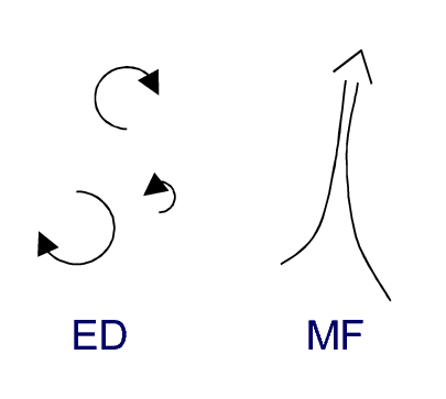
Figure 1. Visualization of the EDMF approach in parameterizing the vertical transport by turbulence and convection in the atmosphere.

Large-scale circulation models used for Numerical Weather Prediction (NWP) and climate simulation are formulated in terms of budget equations for a set of conserved state variables $\phi$ (such as certain definitions of temperature and humidity, and momentum) that usually have the following form, \begin{eqnarray*} \frac{D \phi}{D t} = S_{\phi} \end{eqnarray*} where the left-hand side is the total derivative (including advection) and $S_{\phi}$ represents the collection of sources and sinks that affect $\phi$ over time. The grid-spacings of such global models are typically too large to resolve turbulence and cumulus convection, and as a result the impact of these processes on the larger-scale flow has to be parameterized. These fast-acting processes appear in the budget equation as a flux-divergence term, here simplified to only include the vertical component, \begin{eqnarray*} S_{\phi,tc} = - \frac{\partial \overline{w'\phi'}}{\partial z} \end{eqnarray*} where subgrid $tc$ indicates turbulence and convection, the overline indicates a horizontal Reynolds' average, and the prime a perturbation from this mean. Ever since the advent of numerical simulation of atmospheric flow the closure of the flux $\overline{w'\phi'}$ has been subject to intense research, and many different methods have been proposed. At the foundation of most schemes are two basic transport models. The first is the Eddy Diffusive (ED) transport model which describes the behavior by small-scale turbulent processes, acting to even out differences. \begin{eqnarray*} \overline{w'\phi'}_{ED} \sim - K_{\phi} \frac{\partial \overline{\phi}}{\partial z} \end{eqnarray*} where $K_{\phi}$ is the eddy diffusivity coefficient. As expressed by the dependence on the vertical gradient, in principle this model acts purely down-gradient, and can not penetrate inversions very deeply. The second basic transport model is advective, and describes the behavior of larger-scale convective motions (or plumes) that have enough inertia to overcome stable layers, \begin{eqnarray*} \overline{w'\phi'}_{MF} \approx M_c \left( \phi_c -\phi_e \right) \end{eqnarray*} where $M_c$ is the volumetric Mass Flux (MF) by the convective elements, defined (in approximation) as the product of their area fraction and their vertical velocity. Such motions can transport in counter-gradient directions, and can maintain differences between a convective plume ( c) and its environment (e) for some time. The Eddy Diffusivity - Mass Flux (EDMF) approach is a relatively new method that aims to combine the benefits of both ways of describing transport, \begin{eqnarray*} \overline{w'\phi'} = - K_{\phi} \frac{\partial \overline{\phi}}{\partial z} + M_c \left( \phi_c -\phi_e\right) \end{eqnarray*} This way, both diffusive and advective behavior can be accommodated within one transport scheme, which allows it to deal with more complex situations compared to the two basic transport models alone. In addition, combining ED and MF can also bring some numerical advantages, for example making time integrations more numerically stable. The EDMF concept was first applied to well-mixed layers, such as the clear convective boundary layer (CBL) and the stratocumulus-topped boundary layer. Later EDMF was extended to shallow cumulus topped boundary layers as well as deeper precipitating convection. In all these applications EDMF was coupled to the surface through the plume initialization, often making use of similarity theory to estimate their initial properties.

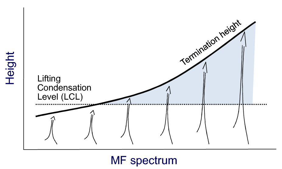
Figure 2. Schematic illustration of an EDMF formulated in terms of multiple plumes. The variation of lifting condensation level and termination height across the spectrum of plumes is indicated by the dotted and solid black lines, respectively.

The original application of EDMF made use of a single bulk MF plume, which then describes the average properties of a whole ensemble of cumulus clouds. However, the bulk plume can also be split up into multiple ones, thus adding “resolution” the MF part of the scheme, \begin{eqnarray*} \overline{w'\phi'} = - K_{\phi} \frac{\partial \overline{\phi}}{\partial z} + \sum_{i=1}^{n} M_i \left( \phi_i -\phi_e\right) \end{eqnarray*} where subscript $i$ indicates the average properties of plume i. This yields a spectrum of plumes, each slightly different, as illustrated in Fig. 2. What each plume represents depends on its definition, for which various options have been proposed. What unites these EDMF versions however is the use of a spectrum of plumes, which enables them to overcome non-linearities that are hard to capture by advective schemes that carry less complexity.

Figure 3. Single Column Model (SCM) results with the multi-plume ED(MF)ⁿ scheme based on discretized size distributions for the RICO shallow cumulus case. Clockwise from the top left: liquid water potential temperature $\theta_l$, total specific humidity $q_t$, and the total area fraction and volumetric mass flux of all condensed EDMF plumes combined. The simulation was performed with ED(MF)ⁿ implemented in DALES as a subgrid scheme, using an ensemble of 10 plumes. DALES was run on an 8×8 grid at grid-spacing of 10km horizontally and 40 m vertically, using a time-integration step of 300 s. More results with the DALES-ED(MF)ⁿ model, also for other cumulus cases, can be found on this QUICKLOOK page.

A benefit of multi plume models is that bulk properties can in principle be diagnosed from the reconstructed spectrum of rising plumes, making classically-used bulk closures obsolete. For example, plumes can condense or not, depending on their proximity to saturation. As a result, the scheme becomes sensitive to environmental humidity, a behavior that recent research has found to be an essential feature in convection schemes. The number of plumes that reach their lifting condensation level and continue as transporting cumulus clouds is automatically found by the scheme itself (see also Fig 2). An environment closer to saturation will yield a higher number of rising plumes that will condense at the top of the mixed layer, which immediately boosts the cloud base mass flux. This allows the scheme to effectively, and swiftly, find the point at which the vertical transport of mass, heat and humidity through cloud base by all plumes together exactly counteracts the effect of the destabilizing large-scale forcings. This situation corresponds to a quasi-equilibrium state, and the feedback mechanism that establishes it is called the shallow cumulus valve mechanism. An advantage of multi-plume MF models is that this process can be captured automatically, yielding smooth simulations for idealized prototype cumulus cases (see Fig. 3).

Multi plume models have also shown skill in capturing transitions between convective regimes. Co-existing plumes, each independently distributing heat and moisture across layers of differing depths, can together effectively deal with situations in which more than one convective mode are active. As a result, phenomena such as the internal decoupling in the boundary layer as well as transitions from stratocumulus to shallow cumulus can be reproduced.

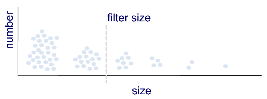
Figure 4. Schematic illustration of a discretized size density of the number of plumes, with number typically decreasing sharply with size. A low-pass size filter introducing scale-adaptivity is indicated by the dashed grey line.

An ensemble of plumes can be differentiated based on updraft properties such as thermodynamic state, vertical velocity or buoyancy. Alternatively one can define a plume spectrum in size-space, as schematically illustrated in Fig. 4. This has some important consequences. For example, the size distribution of plume properties becomes the foundation of the EDMF framework. This can be understood by rewriting the multi-plume MF flux at some height $z$ as a function of plume size $l$, \begin{eqnarray*} \overline{w' \phi'}_{MF}(z) & \approx & \int_{l} \mathcal{M}(l,z) \left[ \phi(l,z) - \phi_e(z) \right] dl \\ & = & \int_{l} \mathcal{A}(l,z) \left[ w(l,z) - w_e(z) \right] \left[ \phi(l,z) - \phi_e(z) \right] dl \label{eq:fluxdensity} \end{eqnarray*} where the calligraphic symbols $\mathcal{A}$ and $\mathcal{M}$ represent the probability density functions of plume area fraction and plume mass flux, respectively. The area density can be further expanded in terms of the size density of plume number, $\mathcal{N}$, \begin{equation*} \mathcal{A}(l,z) = \mathcal{N}(l,z) l^2. \end{equation*} Variable $\mathcal{N}(l,z)$ is also known as the number density of plumes, and acts as a weight in the MF equation; the higher the number of plumes of size $l$, the larger their contribution to the flux. In numerical practice, the integrals have to be replaced with summations. In case a limited number of bins is used to discretize the size distributions, one effectively works with discretized size densities. As these size densities describe the macrophysical properties of the plume ensemble, such schemes can also be called bin macrophysics schemes. The acronym ED(MF)ⁿ stands for a multi-plume EDMF version that makes use of a discretized size density containing n bins.

The size distributions of some variables in the framework also carry a height dependence. These variables include the vertical profiles of area fraction, vertical velocity and the excesses of thermodynamic state and momentum over the environment. The vertical profiles are calculated for each size-bin using the rising plume model. Other size distributions have to be parameterized. The most important one is perhaps the number density of the plumes, but also the size dependence in the lateral mixing rate between plumes of a certain size and their environment needs closure. How to achieve this is subject to ongoing research by the InScAPE group.

Figure 5. Histograms of cloud properties as a function of their size, maintaining height dependence, as diagnosed in an LES of the BOMEX shallow cumulus case. From left to right: vertical velocity $w$, cloud-average condensate $q_l$, and the excess of virtual potential temperature $\theta_v$ over their environment. Cloud size increases from black (50m) via green to brown (600m). The grey line indicates the hypothetical properties of an undiluted condensed plume, for reference. After sorting clouds on their size, defined as the square-root of their height-averaged area fraction, the bin-average properties are calculated.

What motivates the formulation of EDMF in terms of discretized size densities? One reason is that size dependence is often observed in aspects of cumulus cloud populations, in observations but also in LES, as shown in Fig. 5. This also means that individual components of the EDMF can in principle easily be confronted and constrained with relevant observations. A good example of a reliable observable is the cloud number density, which has been investigated for decades using satellite and high-altitude aircraft imagery, and recently also scanning radar imagery.

Figure 6. A schematic illustration of indirect feedback mechanisms between large and small plumes that are active within a bin macrophysics scheme.

Another motivation for introducing size-dependence in the plume ensemble is that it introduces indirect feedbacks between large and small condensed plumes, as revealed by recent research by InScAPE. These feedbacks act through the mean thermodynamic state. As illustrated by Fig. 6, the larger, less diluted condensed plumes tend to accelerate immediately above cloud base, due to significant latent heat release associated with condensation. The locally strong drying and cooling tendency resulting from this increase of flux with height is counteracted by the detrainment by smaller, weaker plumes that terminate above their LCL. This way, the ensemble of plumes cooperates to automatically create the flux profiles that exactly balance the large-scale forcings in the cloud layer. This cooperation has been named the “acceleration-detrainment” mechanism, and is captured by the ED(MF)ⁿ scheme.

Another clear benefit of the formulation of the ED(MF)ⁿ transport scheme in size-space is that it creates opportunities for introducing scale-adaptivity in a natural way, at the foundation of the framework. This can be achieved by filtering out the contribution to the vertical flux by all plumes larger than a certain size-threshold, proportional to the horizontal grid spacing of the host circulation model. This concept is illustrated in Fig. 4. As a result, the activity of the EDMF as a subgrid scheme will be gradually reduced when simulations are performed at a higher horizontal resolution. This means that the scheme becomes scale-adaptive.

The question is then how the resolved scales will respond to the scale-adaptivity introduced in ED(MF)ⁿ. It can be expected that, when performing simulations at ever higher resolution with this framework, at some point resolved turbulence and convection will appear. This has to happen, as instability (created continuously at a slow rate by the larger scale forcings) will have to be overturned somehow. This point, at which the resolved and unresolved scale both contribute in a roughly equal measure to the total vertical distribution, is called the grey zone of boundary layer convection. Usually, for shallow cumulus, this zone is situated somewhere around 500m. However, in numerical practice this point is likely to be dependent on the subgrid-scheme that is used.

Figure 7. Illustration of the under-sampling of a cloud size distribution as a result of a too small GCM gridbox size. Left panel: the cloud mask (in black) in a 2D snapshot from a LES realization of the RICO shallow cumulus case. The domain size is 51.2×51.2 km, at a resolution of 25m. The boxes in red represent three different GCM gridboxes. Right panel: The normalized size density of the number of clouds in the largest domain, illustrating the effect of subsampling on the right tail of the distribution. The dashed line is a powerlaw-exponential fit.

While the introduction of scale-adaptivity is a step in the right direction, this does not solve another problem that is introduced by the ever increasing resolutions in GCMs. This is the appearance of stochastic behavior as a result of the under-sampling of a cumulus cloud population. As illustrated by Fig. 7. cumulus cloud populations consist of many clouds of different sizes, including many small clouds but few large clouds. The spacing between the clouds typically is proportional to their size. When the domain size in which the population is considered is too small, too few large clouds are sampled to obtain a stable distribution that matches the true distribution. In other words, the sample size is too small. As a result, sampling the cloud size distribution (CSD) at a later point will yield a different CSD, with the main deviations or “noise” at the larger end of the tail. This stochastic behavior also has to be represented somehow in the scheme.

Answering these research questions is one of the main research goals of the InScAPE group.

DALES-ED(MF)ⁿ basically stands for the DALES code with the ED(MF)ⁿ scheme implemented as a subgrid scheme, replacing the original Sub-Filter Scale (SFS) scheme (Smagorinsky or TKE). Results with this scheme for a set of well-known prototype cumulus cases are provided on this QUICKLOOK page. All simulations were performed on a 8×8 microgrid with dx=dy=10 km and dt=300 sec.

The cases for which the scheme is tested cover different climate regimes and convective types. Marine subtropical shallow cumulus conditions are described by the RICO and BOMEX case. Continental diurnal cycles of shallow cumulus are represented by the classic “ARM SGP” case (21 June 1997), various LASSO cases, and selected days at the mid-latitude JOYCE site in Germany. Transitional cases from stratocumulus to cumulus include the ASTEX case and the SLOW, REFERENCE and FAST case as described by Sandu et al., all of which featured in the recent SCM intercomparison study by Neggers et al. (2017) as part of the EUCLIPSE project. Finally, deep convective conditions are covered by the humidity-convection case of Derbyshire et al (2004) and a variation of the BOMEX case with modified surface fluxes described by Kuang and Bretherton (2000).

For more information get in contact with Roel Neggers.