Table of Contents
Data evaluation
Rain gauges
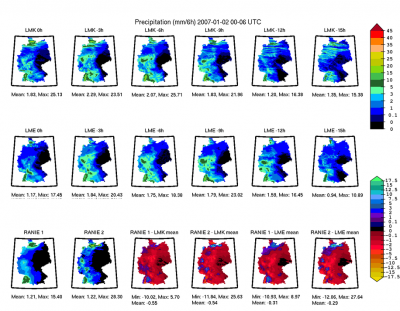
- Daily quicklooks for each 6 h RANIE interval
- Monthly evaluation of daily precipitation sums for corresponding LMK gridpoints
- Timing of precipitation events for high temporal resolution sondes
- Statistical analysis for specific regions
Radio soundings:
Plots for each sounding in Germany and neigbouring countries
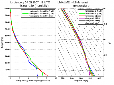
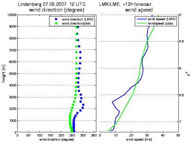
- Stüve diagramm together with corresponding +12h LMK forecast
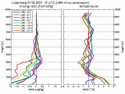
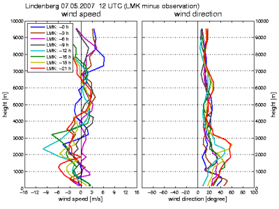
- differences of temperature, specific humidity, wind speed and wind direction forecasts (-0,-3,-6,-9,-12,-15,-18,-21 h) at each model level
Monthly statistics
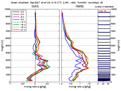
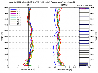
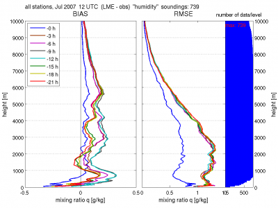
- Bias and RMS profiles for temperature, humidity and wind for all stations
Mean BIAS and RMSE of temperature, humidity and wind speed of all available radio soundings for each station and month. The diagram on the right side of the pictures (blue horizontal bars) shows a statistic of the data, which are available for each model level.
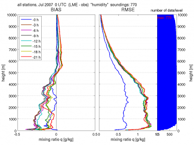
Mean of all stations (delta z = 50 meters)
Mean BIAS and RMSE of all soundings of all stations together for each month. To compare the stations we had to average the model data and the observations to levels with 50 m vertical spacing, because every station has a different height and the model levels are located in different heights above sea level (dependent on the geographical height). We have created statistics of all available soundings of 12 UTC, 0 UTC and all together (0,6,12,18 UTC) for each month. The “blue” diagram on the right side of each picture shows a statistic of the data, which are available for each 50 m level. It is the same as in the statistic above but with much more levels.
Ceilometer
DWD ceilometer network of about 100 stations as well as auxillary stations (Bonn, Cabauw, Lindenberg..)
- Daily colour coded maps (see GPS example) of BIAS/RMS/correlation of cloud base height (LMK vs observation)
- Monthly time series of Bias/RMS for each station or region (depending on number of stations within regions)
- Monthly analysis of mean diurnal cycle and comparison to differnet model runs (lagged ensemble)
- Statistical comparison of mixing height overthe full year for EARLINET stations
- Statistics of aerosol distribution for EARLINET stations
GPS
Comparison of the GPS iwv to COSMO-DE and COSMO-EU
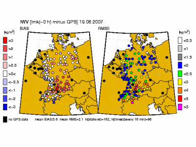
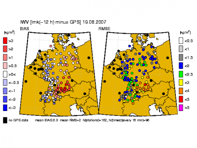
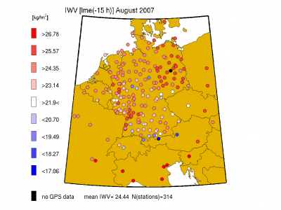
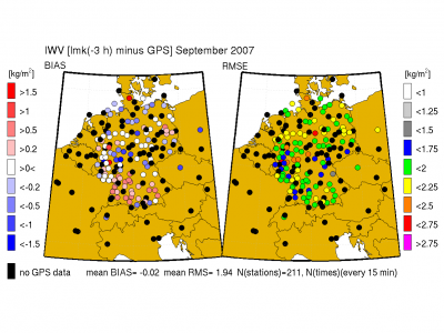
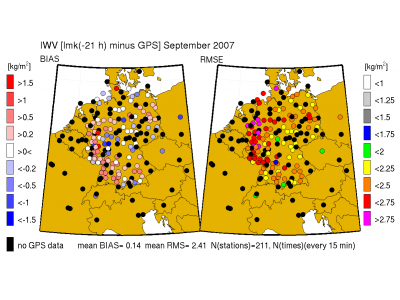
- Daily colour coded maps of BIAS/RMS/correlation of integrated water vapor (IWV) (model vs observation)
Daily maps of BIAS and RMSE [COSMO-DE and COSMO-EU IWV (grid point near each station) minus IWV of each GPS-station] of all model forecasts -0 h,-3 h,-6 h,-9 h,-12 h,-15 h,-18 h,-21 h before the measurements.
monthly statistics
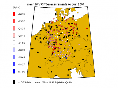
Mean IWV (models and observations)
Monthly averaged IWV of observations and monthly averaged IWV of COSMO-DE and COSMO-EU (grid point near each station) of all model forecasts (-0 h,-3 h,-6 h,-9 h,-12 h,-15 h,-18 h,-21 h) before measurements.
Mean Bias and RMSE
Maps of monthly averaged BIAS and RMSE [COSMO-DE and COSMO-EU IWV (grid point near each station) minus IWV of each GPS-station] for all model forecasts -0 h,-3 h,-6 h,-9 h,-12 h,-15 h,-18 h,-21 h before the measurements.
Statistics of all stations together
Monthly and for several specific times : The times are not randomly chosen. The models (COSMO-DE and COSMO-EU) have changed between these times.
For the monthly statistics and the specific times you can choose between:
- “all available stations and time steps for COSMO-DE and COSMO-EU” and
- “the same stations and time steps for COSMO-DE and COSMO-EU”
Some GPS stations are outside of the COSMO-DE area. For comparison between the two different models the locations have to be the same. COSMO-DE creates a model output every 15 minutes. COSMO-EU only every hour. For the statistics it is important to average about the same number of data and to compare the same timesteps. So 1. is good for comparison between different runs of the respective model because all available data are considered and 2. is good for comparison between COSMO-DE and COSMO-EU.
Mean BIAS and RMSE
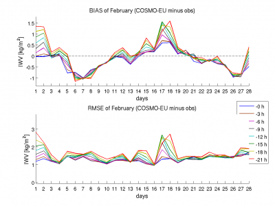
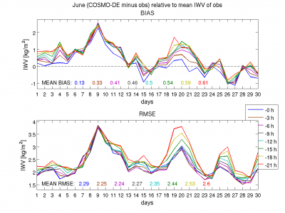
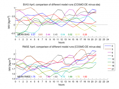
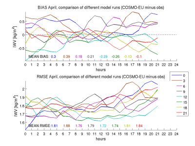
The pictures show a time series of BIAS and RMSE of each model and observation, averaged over all stations every timestep. The different colors present the different forecasts of the model dependent on the starting time of the model run before each measurement of the IWV.
Diurnal Cycle, Mean Bias and RMSE
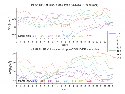
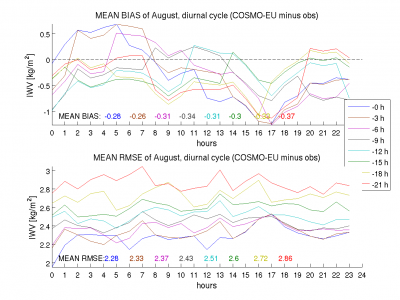
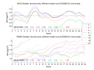
The pictures show the diurnal cycle of BIAS and RMSE of the respective model and observations, averaged over all stations and time of day. The different colors present the different forecasts of the model dependent on the starting time of the model run before each measurement of the IWV.
Diurnal Cycle of different model runs, Mean BIAS and RMSE
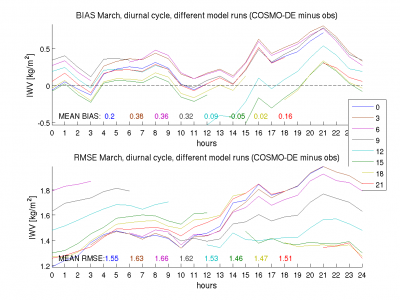
The pictures show the diurnal cycle of BIAS and RMSE of the respective model and observations, averaged over all stations and time of day. Here the different colors present the different model runs dependent on the starting time of each model run. But here for example the red line does not present the forecast of 21 hour before each measurement as in the statistics above. It presents the average chronological sequence of the Bias of model run started at 21 UTC. The model runs are compared with the corresponding measurements and so each picture describes the development of each model run.
Comparison of different model runs, Mean BIAS and RMSE
It is the same statistic as described above but here the abscissa does not present the daytime. It describes the lead time of each model. So all averaged “BIAS-runs” start at 0 and you can compare much better.
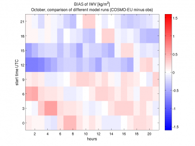
Comparison of different model runs, Mean BIAS and RMSE (MATRIX-Plots)
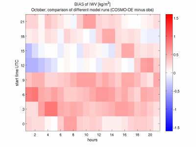
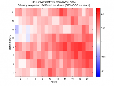
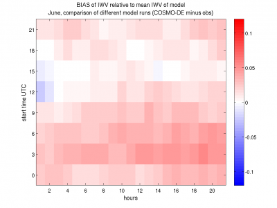
The pictures present the same as above but it is another demonstration of the results of the BIAS. The numbers at the ordinate stand for the starting time of the model runs. The numbers at the abscissa stand for the lead time of the respective model run. Red rectangles depict a positive BIAS and blue rectangles depict a negative BIAS. The horizontal distribution represents the development of the averaged “BIAS-runs”. When you follow the rectangles diagonal you can compare the averaged BIAS of the model runs at equal day times.
Comparison of different model runs, Mean BIAS and RMSE relative to mean IWV of model (MATRIX-Plots)
The difference to the statistic above is the division by the mean IWV of the respective month. The IWV values of the summer months are much greater than the values of winter months and of course the values of BIAS and RMSE too. So the division by the mean IWV is necessary if you want to compare the results of different months.
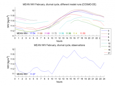
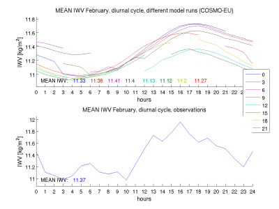
Diurnal Cycle of different model runs, Mean IWV
The statistics described before allways present the BIAS and RMSE, so the comparison of model and observations. This statistic shows the diurnal cycle of the pure IWV of the different model runs and the observations separately. Note that the averaged IWV of observations and model runs were computed over a different number of data so you can hardly compare them.
- Monthly time series of Bias/RMS for each station or region (depending on number of stations within regions)
- Monthly analysis of mean diurnal cycle and comparison to differnet model runs (lagged ensemble)
Micro Rain Radar (MRR)
- Daily plots of time-height distribution of rain water from LMK and MRR for about 11 stations in Germany
- Monthly analysis of vertically resolved rain water BIAS/RMS/correlation for all MRR stations
- Analysis of brightband height
- Yearly mean diurnal cycle of rain water
RADAR
- daily maps of the precipitation sums
- time series for the various regions
- time series at mrr stations
- statistics:
- mean precipitation rate per area
- percentage of the area with precipitation
- for each day the pdf
- same plots for the model data
Satellite
SEVIRI / Meteosat
- Quicklooks for every 15 min available at FU Berlin (Europe)
- True Color Image (TCI)
- Cloud Mask (CM)
- Clear sky Brightness temperature at 10.8 µm
- Integrated Water Vapor (IWV)
- Cloud Top Pressure (CTP)
- Time series of satellite products and model forecast at selected stations (exact column and mean value of 3×3 grids)
- brightness temperatures for all 8 IR MSG channels
- cloud mask, cloud fraction, optical depth, IWV, CTP
- Statistics (MSG and model) for the various areas at 15 min resolution (see below)
- Mean, median and standard deviation of brightness temperatures for all 8 IR MSG channels
- pdf (20 classes, min=180, max=350) for each of the 8 R MSG channels
- Mean cloud coverage and mean cloud free coverage
- pdf (20 classes, min=0, max=1) of the cloud probability
- Mean, median and standard deviation of cloud top pressure
- pdf (20 classes, min=0, max=1000) of the cloud top pressure
- Mean, median and standard deviation of optical depth
- pdf (20 classes, min=0, max=200, logarithm) for optical depth
MERIS
- Quicklooks available at FU Berlin
- True Color Image (TCI)
- Cloud Mask (CM)
- Cloud Top Pressure (CTP)
- Cloud Optical Thickness (COT)
- Integrated water vapour (IWV)
- Time series of satellite products and model forecast at selected stations
- Maps for GOP area of model and satellite
MODIS
- Maps of satellite overpasses for GOP area and corresponding model forecasts
- Cloud Mask (CM)
- Cloud Optical Thickness (COT)
- Integrated water vapour (WV)
- Cloud top pressure (CTP)
- Effectiv particle radius (REFF)
- Time series of satellite products and model forecast at selected stations
- Maps for GOP area of model and satellite
Areas for the evaluation:
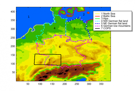
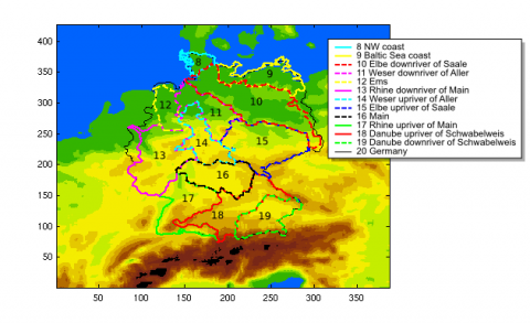
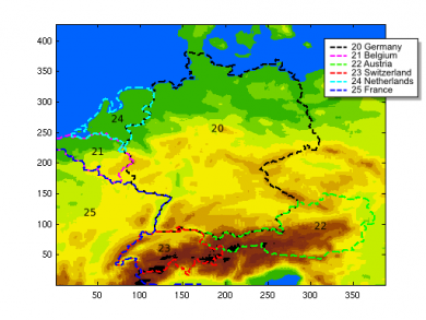
There are 25 areas for the evaluation which are made up of 7 geographic areas, 12 river catchments in Germany and 6 countries.
| No. | Name | Code | Type/Definition |
|---|---|---|---|
| 1 | North Sea | nort | geographic area: water west of Denmark |
| 2 | Baltic Sea | balt | geographic area: water east of Denmark |
| 3 | Alps | alps | geographic area: mountains higher than 700 m |
| 4 | NW German flat land | nwgf | geographic area: North Germany below 200 m and west of x = 205 |
| 5 | NE German flat land | negf | geographic area: North Germany below 200 m and east of x = 205 |
| 6 | German low mountains | glmo | geographic area: Germany above 200 m |
| 7 | COPS | cops | geographic area: Rectangle 6° - 10° E and 47.7° - 49.2° N |
| 8 | NW coast | nwco | river catchment: northern coastal areas of northernmost Germany |
| 9 | Baltic Sea coast | bsco | river catchment: Baltic Sea coast |
| 10 | Elbe downriver of Saale | elds | river catchment: Elbe downriver of Saale |
| 11 | Weser downriver of Aller | weda | river catchment: Weser downriver of Aller |
| 12 | Ems | emsc | river catchment: Ems |
| 13 | Rhine downriver of Main | rhdm | river catchment: Rhine downriver of Main |
| 14 | Weser upriver of Aller | weua | river catchment: Weser upriver of Aller |
| 15 | Elbe upriver of Saale | elus | river catchment: Elbe upriver of Saale |
| 16 | Main | main | river catchment: Main |
| 17 | Rhine upriver of Main | rhum | river catchment: Rhine upriver of Main |
| 18 | Danube upriver of Schwabelweis | dous | river catchment: Danube upriver of Schwabelweis |
| 19 | Danube downriver of Schwabelweis | dods | river catchment: Danube downriver of Schwabelweis |
| 20 | Germany | germ | country |
| 21 | Belgium | belg | country |
| 22 | Austria | aust | country |
| 23 | Switzerland | swit | country |
| 24 | Netherlands | neth | country |
| 25 | France | fran | country |
For COSMO model output area statistics, additionally the following areas are considered:
| No. | Name | Code | remark |
|---|---|---|---|
| 26 | COSMO-DE area (without 20 boundlines) | code | |
| 27 | AMF_Murgtal 3×3 gridpoints | am03 | |
| 28 | Beauvechain 3×3 gridpoints | bv03 | |
| 29 | Bergen-Hohne 3×3 gridpoints | bh03 | |
| 30 | Cabauw 3×3 gridpoints | ca03 | |
| 31 | COPS_Supersite_H 3×3 gridpoints | ho03 | |
| 32 | COPS_Supersite_R 3×3 gridpoints | rh03 | |
| 33 | COPS_Supersite_S 3×3 gridpoints | st03 | |
| 34 | Emden-Koenigspolder 3×3 gridpoints | em03 | |
| 35 | Essen-Muelheim 3×3 gridpoints | es03 | |
| 36 | Lichtenau 3×3 gridpoints | ln03 | |
| 37 | Lindenberg 3×3 gridpoints | lb03 | |
| 38 | Nancy-Essey 3×3 gridpoints | na03 | |
| 39 | Payerne 3×3 gridpoints | py03 | |
| 40 | AMF_Murgtal 9×9 gridpoints | am09 | |
| 41 | Beauvechain 9×9 gridpoints | bv09 | |
| 42 | Bergen-Hohne 9×9 gridpoints | bh09 | |
| 43 | Cabauw 9×9 gridpoints | ca09 | |
| 44 | COPS_Supersite_H 9×9 gridpoints | ho09 | |
| 45 | COPS_Supersite_R 9×9 gridpoints | rh09 | |
| 46 | COPS_Supersite_S 9×9 gridpoints | st09 | |
| 47 | Emden-Koenigspolder 9×9 gridpoints | em09 | |
| 48 | Essen-Muelheim 9×9 gridpoints | es09 | |
| 49 | Lichtenau 9×9 gridpoints | ln09 | |
| 50 | Lindenberg 9×9 gridpoints | lb09 | |
| 51 | Nancy-Essey 9×9 gridpoints | na09 | |
| 52 | Payerne 9×9 gridpoints | py09 | |
| 53 | LMQ area (without 20 boundlines) | lm_q | for COSMO-EU only |
| 53 | AMF_Murgtal 25×25 gridpoints | am25 | for COSMO-DE only |
| 54 | Beauvechain 25×25 gridpoints | bv25 | for COSMO-DE only |
| 55 | Bergen-Hohne 25×25 gridpoints | bh25 | for COSMO-DE only |
| 56 | Cabauw 25×25 gridpoints | ca25 | for COSMO-DE only |
| 57 | COPS_Supersite_H 25×25 gridpoints | ho25 | for COSMO-DE only |
| 58 | COPS_Supersite_R 25×25 gridpoints | rh25 | for COSMO-DE only |
| 59 | COPS_Supersite_S 25×25 gridpoints | st25 | for COSMO-DE only |
| 60 | Emden-Koenigspolder 25×25 gridpoints | em25 | for COSMO-DE only |
| 61 | Essen-Muelheim 25×25 gridpoints | es25 | for COSMO-DE only |
| 62 | Lichtenau 25×25 gridpoints | ln25 | for COSMO-DE only |
| 63 | Lindenberg 25×25 gridpoints | lb25 | for COSMO-DE only |
| 64 | Nancy-Essey 25×25 gridpoints | na25 | for COSMO-DE only |
| 65 | Payerne 25×25 gridpoints | py25 | for COSMO-DE only |
Area Statistics
Mean:
soil temperature, soil water, canopy water, surface snow amount, vertical velocity in 5000 m, 3000 m, 2000 m, 1500 m, 1000 m, 500 m, relative humidity, omega, geopotential, and horizontal wind components in 300 hPa, 500 hPa, 700 hPa, 850 hPa, 950 hPa, temperature in 300 hPa, 500 hPa, 700 hPa, 850 hPa, 950 hPa, 1000 hPa.
Mean, minimum, maximum:
surface pressure, mean-sea-level pressure, 2-m temperature, 10-m (lowest model level) temperature, 10-m (lowest model level) specific humidity, soil surface temperature, surface temperature, surface specific humidity, surface runoff, subsurface runoff, averaged surface net downward shortwave radiation, averaged surface net downward longwave radiation, averaged surface sensible heat flux, averaged surface latent heat flux, surface evaporation, u_10m, v_10m, windspeed_10m; constant variables: land area fraction, root depth, vegetation area fraction, leaf area index.
Mean, minimum, maximum, median, standard deviation:
total water content, vertically integrated cloud ice, vertically integrated cloud water, atmospheric boundary layer height (above msl), CAPE (parcel ascent from lowest model level, contributions from positive buoyancy only), CAPE_CON (only COSMO-EU), CAPE_ML (only COSMO-DE); constant variable: model surface height.
Mean, minimum, maximum, median, standard deviation, frequency distribution:
total cloud cover, cloud cover of high clouds, cloud cover of medium clouds, cloud cover of low clouds, precipitable water (IWV), vertically averaged vertical velocity, vertically averaged absolute wind velocity, total precipitation amount, gridscale rain, gridscale snow, gridscale graupel (COSMO-DE only), convective precipitation amount (COSMO-EU only), gridscale rainfall rate (COSMO-DE only), gridscale snowfall rate (COSMO-DE only), gridscale graupelfall rate (COSMO-DE only), height of convective cloud base, height of convective cloud top, cloud (>0.01) base height, cloud (>0.5) base height, cloud (gridscale only) base height, gridscale liquid-water cloud base height, cloud optical thickness (several methods), cloud top pressure (several methods), SynSat MSG brightness temperature, radar reflectivity in 850 hPa (COSMO-DE only), column maximum radar reflectivity (COSMO-DE only).
Mean, frequency distribution in 72 bins from 0.0 to 360.0:
wind direction in 10 m, 300 hPa, 500 hPa, 700 hPa, 850 hPa, 950 hPa.
Frequency distribution in 13 bins from 0 to 12:
Beaufort in 10 m.
Frequency distribution in 9 bins:
constant variable: soiltyp.
One netcdf file per model (COSMO-DE/COSMO-EU) each with all forecasts valid for all areas for a particular day. Variable names in netcdf file are mostly analogue to those in the COSMO model.
For full information see example output of netcdf -h:
arst_lmk_ncdump.ps for COSMO-DE.
arst_lme_ncdump.ps for COSMO-EU.
;– Susanne Crewell 2007/01/10 14:41

