Wind lidar @ Joyce
raw data from the halo photonics stream line wind lidar in Jülich
The instrument performs several scanning patterns and uses the remaining time for vertical staring.
Resolution is:
- temporal: 1.67 seconds in vertical staring mode. For the scan patterns, it depens on the scanner to reach new positions.
- spatial: 30m
Scan patterns are currently:
- every 5 minutes doppler beam swinging (DBS) (12×14sec/hour=2min48sec/hour)
i.e. one vertical and two tilted beams in eastern and western direction to derive instantaneous local wind profiles
- directly followed by a 3 beam VAD (VAD-3) (12×14sec/hour=2min48sec/hour)
i.e. three tilted beams in at 0, 120 and 240 deg azimuth and 30deg zenith distance to derive instantaneous local wind profiles
- every 15 minutes a velocity azimuth display scan (VAD-36) (4×124sec/hour=8min16sec)
i.e. a conical scan at 75oelevation to derive area averaged wind profiles
- every 60 minutes a range height indicator (RHI) (1×10⁴sec/hour=1min44sec/hour)
i.e. a vertical section from east to west with 5deg elevation steps (37beams)
- the rest of the time is vertical staring, i.e. vertical staring is interrupted every 5 minutes and sums up to 47minutes
An error estimate for the wind profiles can be found here.
Plots of current data:
current wind profile
wind profile from 3 different scans
VAD-plots
time height sections
w-statistics
hodograph
profiles
error and noise behaviour
technical data
VAD-36 scan
rhi scan
See also the Met-data from Jülich
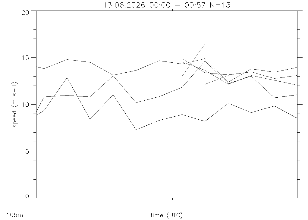
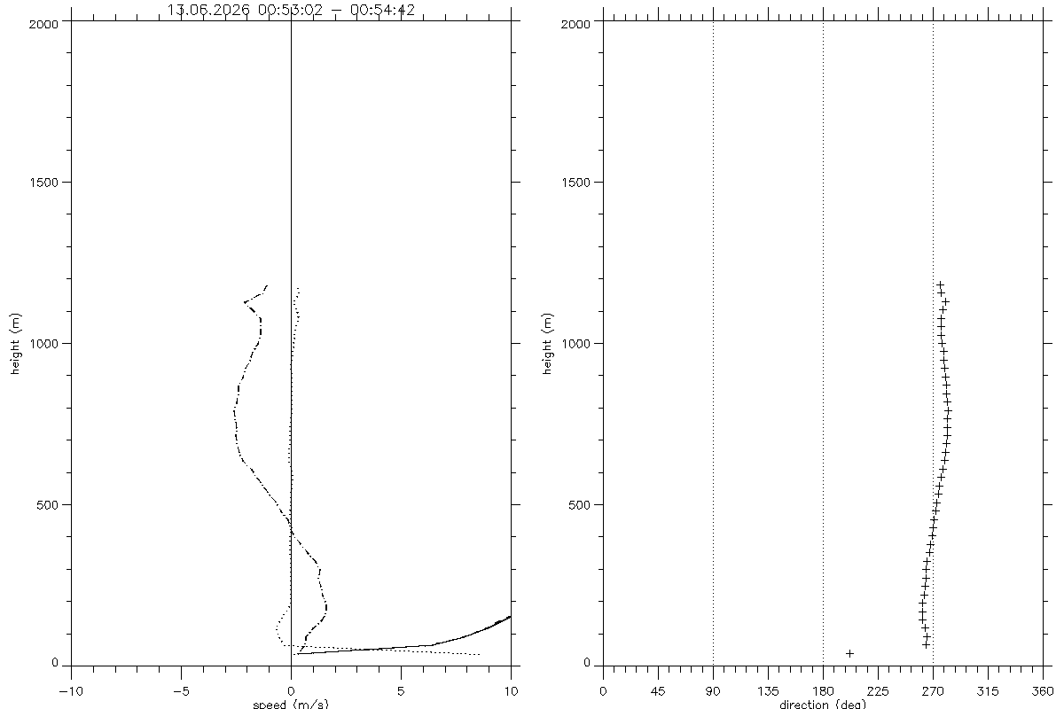
Average profiles from DBS: speed on the left with solid=average, dashed=+/-stddev, dotted=min/max, dash-dotted=last,
direction on the right with large '+' symbol for the average, medium size '+' for average plus, minus stddev and tiny '+' for minimum and maximum.
Last profiles from DBS (left), VAD-3 (middle) and VAD-36 (right):
In every of these plots you find:
left: wind speeds with horizontal speed (thick black) with error bars indicating
total error (black), error from separation (magenta), error from doppler retrieval uncertainty (cyan)
and an error estimate from the residuum of the retreival fit (grey).
The red lines indicate vertical wind from scan retrieval (solid red) and the stddev of the vertical wind (dashed red)
middle: wind direction with error bars (black symbols) and doppler speed at the respective angle (gray lines). Refer to the axes in the upper part of the plot.
right: average backscatter with stddev.
For a comparison of wind retrievals from different subsets of the VAD-36 scan see vad_profiles.html
Click on images so enlarge
Profiles:
Left: thin lines: doppler components along beams in eastern, norhtern and vertical direction (dashed, dash-dotted and dotted)
thick lines: horizontal components in eastern (dashed) and northern direction (dash-dotted)
solid line and +-symbols: horizontal speed from instrument and from own calcualtion.
center: wind direction, +-symbols from instrument and x-symbols from own calcualtion
right: backscatter coeficient in vertical beam.
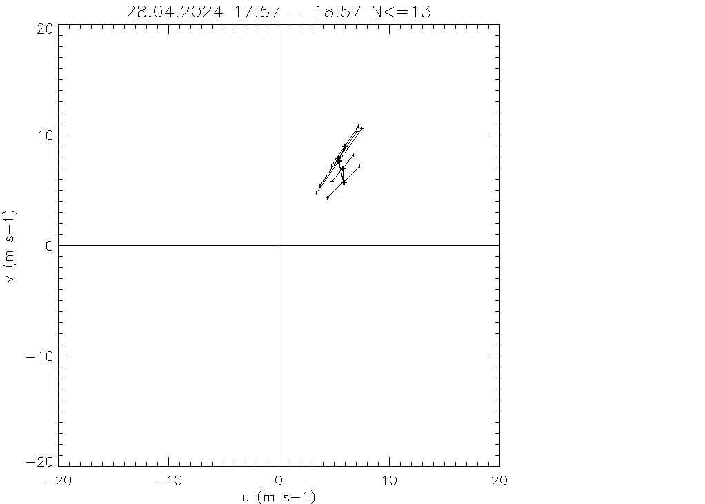
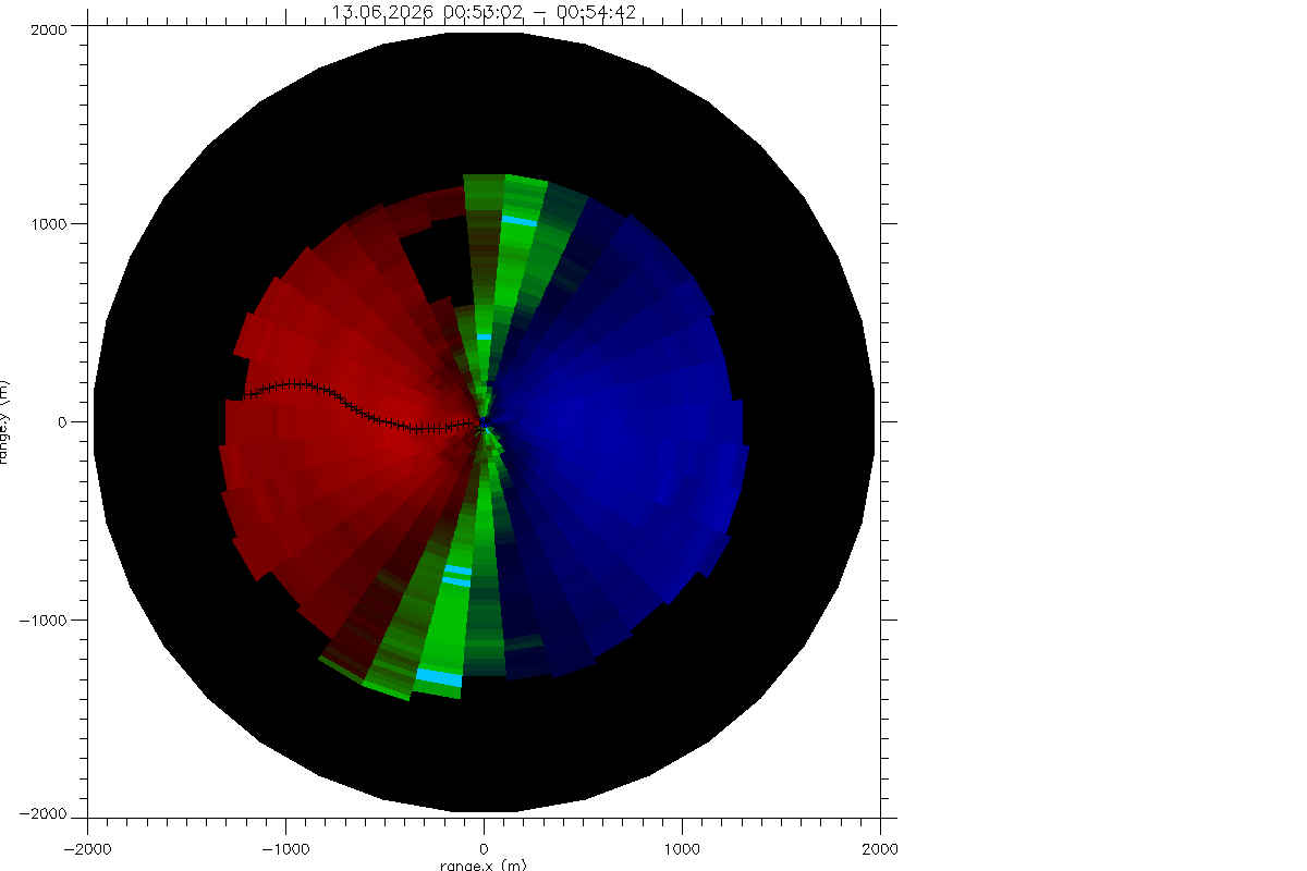
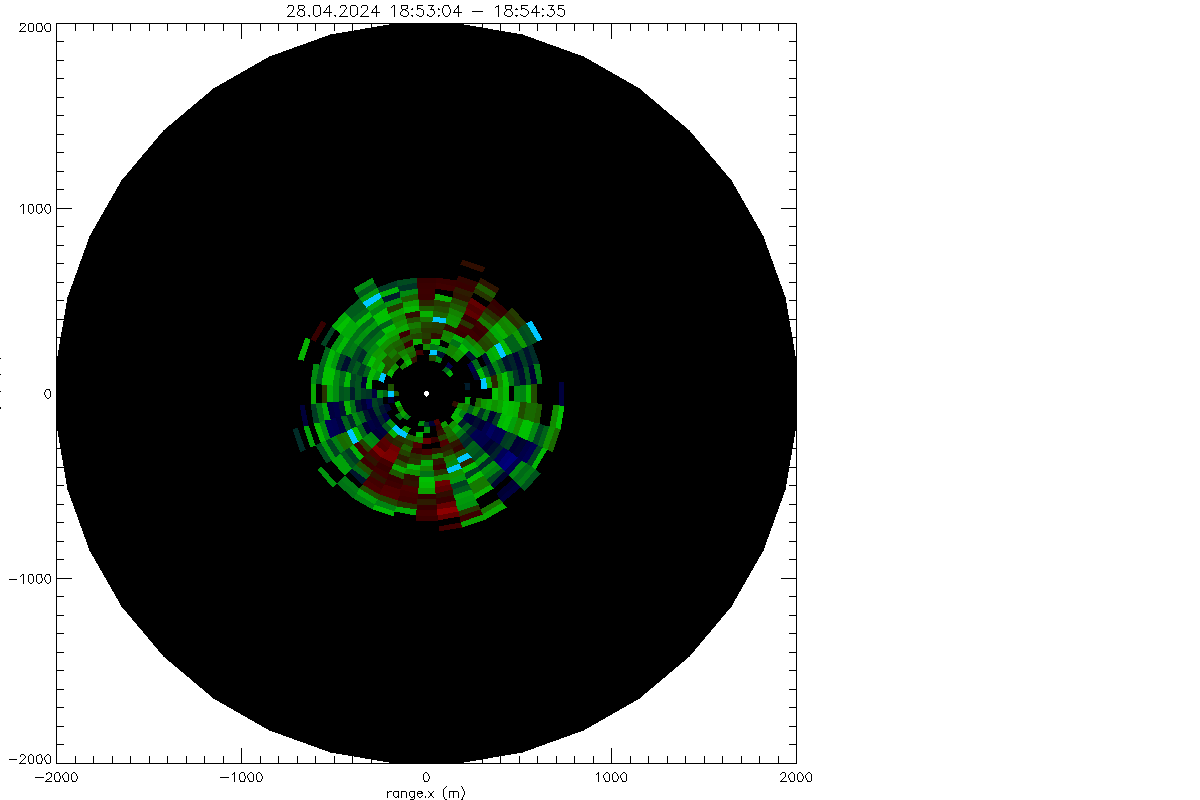
Velocity azimuth display (VAD): vectors give direction and speed of horizontal wind at time and height.
Vectors pointing upward indicate south wind, vectors pointing to the right indicate west wind.
Color shading gives the backscatter coefficient.
Wind vectors are determined by the instrument using the 'beam swing method', i.e. doppler velocities from three
beams are analysed to derive the three componentents of the wind vector at each level. Two of these beams
are tilted at an elavation of 75° and azimuth 0°(north) and 90° (east) and give the wind direction.
A third beam is vertical giving vertical velocity and thus can be used to calculate horizontal velocity from
the tilted beams.
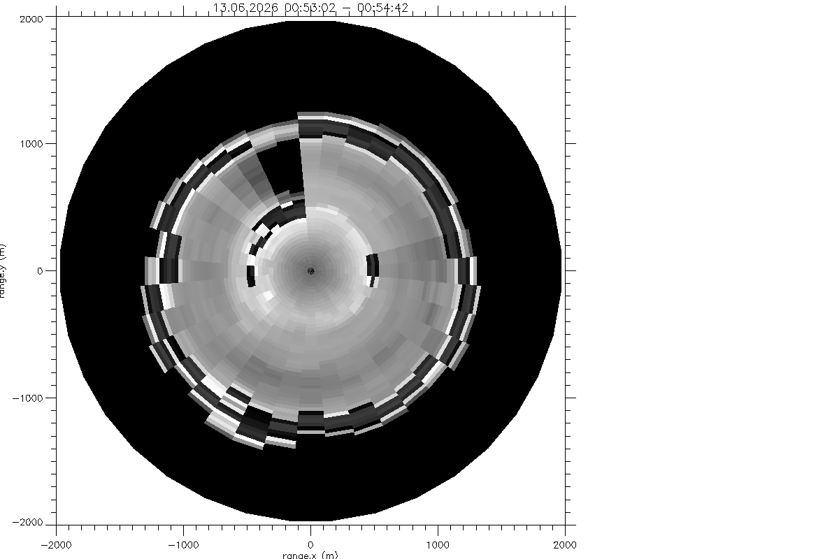
VAD as above for 00-24UTC from VAD-36 scans (left) and dbs scans (right).
The VAD-scan should not be mixed up with the VAD-plot:
The VAD-scan is a scan technique to measure wind profiles with a doppler profiler, the VAD-plot
shows horizontal wind vectors as function of time.
Time - height section of windspeed and direction in one colorcode.
speed vs time
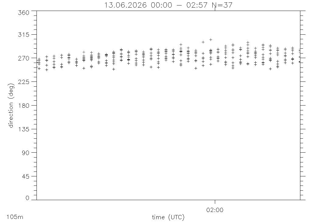
dir vs time
Time height section of vertical wind speed in the lower 2km.
Gaps are due to wind profile measurements by DBS and VAD-3 (every 5 minutes)
and conical scans for the VAD-36 technique (every 15minutes).
log(beta).
Gaps are due to wind profile measurements by DBS and VAD-3 scans every 5 minutes
and conical scans for the VAD-36 every 15 minutes.
Raw Time-height section of intensity. Data here is plotted versus index, gaps from above thus appear here as one pixel columns only.
Raw Time-height section of beta. Data here is plotted versus index, gaps from above thus appear here as one pixel columns only.
Raw Time-height section of log(intensity-1). Data here is plotted versus index, gaps from above thus appear here as one pixel columns only.
Raw Time-height section of log(beta). Data here is plotted versus index, gaps from above thus appear here as one pixel columns only.
Raw Time-height section of vertical wind speed. Data here is plotted versus index, gaps from above thus appear here as one pixel columns only.
'Bad' doppler values, i.e. values that are rejected due to intensity lower than threshold (~1.006)
Vertival velocity (blue = down, red = up) (left) and its histogram (right).
1 sec orignal values of vertival velocity (blue = down, red = up)
Standard deviation of vertival velocity σw in color shading and backscatter coefficient as isolines (left) and its pdf (right).
Standard deviation of vertival velocity σw without (left) and with (right) lag 0 noise correction (left).
Integral euler time scale Tcorr (left) and resulting length scale Lcorr= σwTcorr (right)
Skewness of vertival velocity: without (left) and with (middle) the Lenschow et al 2000 noise correction and the histogram (right, of the not denoised).
Backscatter coefficient (β) (left) and its histogram (right).
Pseudo trajectories calculated from the the high pass filtered vertical wind speed:
zt(t,z0) = z0 + ∫t0t w(zt(t'),t')-wm(zt(t'),t') dt'.
with wm(z,t') = the half hour average of the vertical wind speed.
Hodograph from average wind of the DBS-3 scans with stddev and min,max for speed and direction...
Hodografs from last DBS- (left), VAD-3- (middle) and VAD-36-scan (right):
In every of these plots you find:
left: wind speeds with horizontal speed (thick black) with
total-error (black 2D error-bars),
error from separation (magenta 2D error-bars)
and sigma_w (red circles)
right: traces of the beams in the moving air at different heights (black:z=75m, gray:z=2.5km)
in absolute coordinates (bottom right)
in relative coordinates normalized with correlation length (top right)
Intensity profile
Beta profile (lefdt) and its moments (right):
Variance (solid), skewness (dotted) and Kurtosis (dashed).
log(beta) and its moments variance, skewness and kurtosis (solid, dotted, dashed)
Vertical wind speed and its moments variance, skewness and kurtosis (solid, dotted, dashed)
Vertical wind speed histograms with mean (solid) and median (dotted) marked.
Backscatter coefficient histograms, for all data (black), updrafts (red) and downdrafts (blue). Mean and median are marked solid and dotted respectively.
Top left: Profiles of noise (squares), standard deviation (diamonds) and maxium of w (triangles).
Top right: profile of broadband SNR.
Bottom left: noise versus broadband SNR.
Bottom right: max(w) vs broadband SNR.
Noise is estimated by extrapolating the autocovaraince function from lag 1 to lag 0 (Lenschow et al. 2000).
Standard deviation is corrected for this by substracting the noise.
Solid line in lower left plot shows error estimate after Pearson et al. (2009),
dashed line is the error estime for a direct detection,
horizontal dotted line is standard devation of white noise in full bandwidth interval.
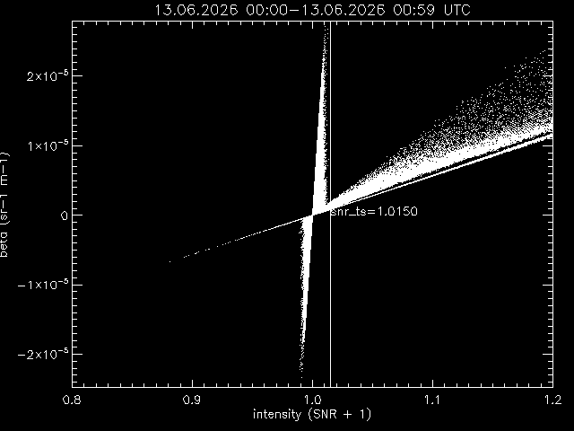
Beta versus intensity
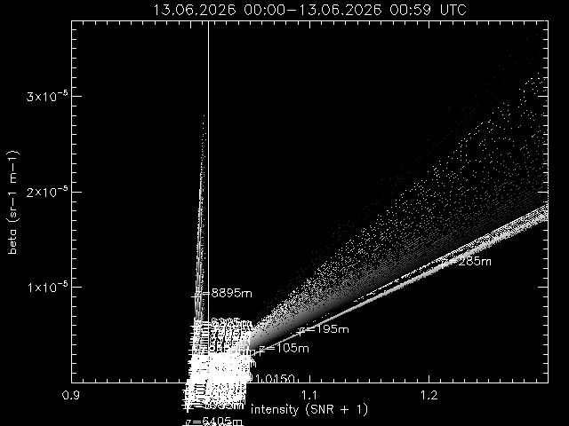

Only positive beta values versus intensity, left linear, right logarithmic
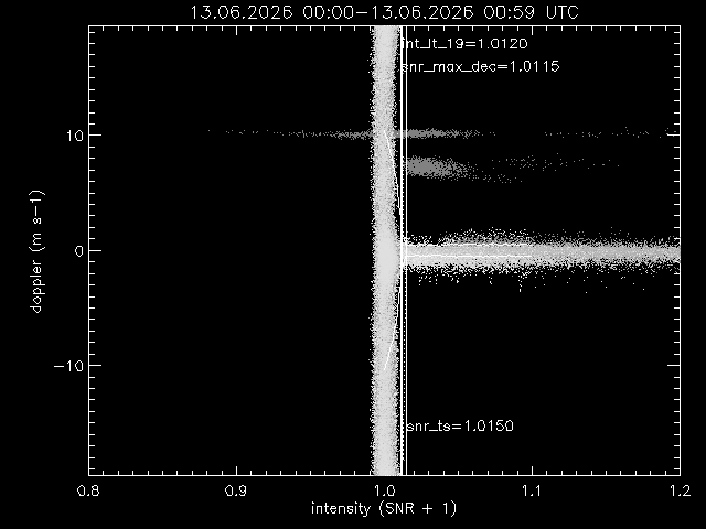
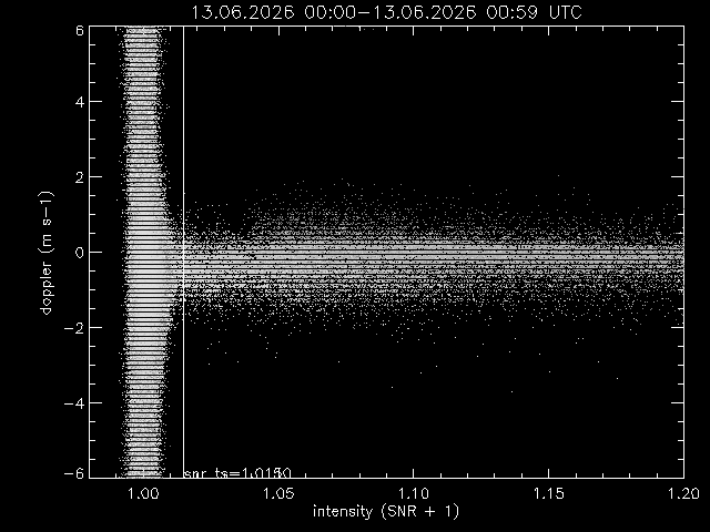
Vertical wind speed versus intensity
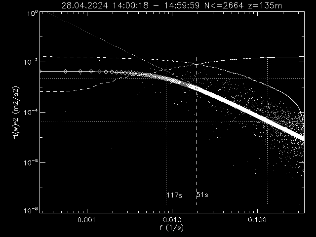
Power spectrum of vertical velocity (dots) and fitted P(f) = 2 P0 /( 1 + (f Tstar)^n ) with n=5/3 (line with diamonds)
Normalized ogives from low to high frequencies and the resulting time/frequency scale
which separates the spectrum at half total power (dashed lines).
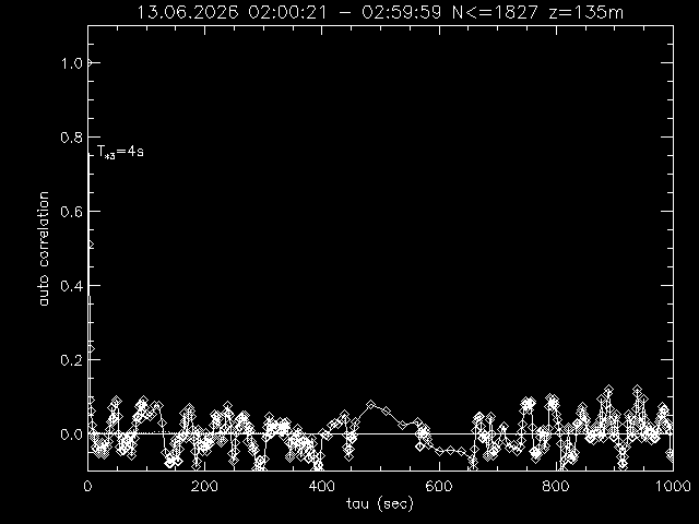
Autocorrelation function with a=exp(-t/T*) fitted to first 10 values (solid), integral ∫0t acor(t') dt'/1000s (dotted)
Background vs time and 'height' (top), and Intensity values around 1 (bottom)
Background vs time (top) and vs range gate (=height) (bottom)
Background values after the pulse (red) and second pulse (blue).
Colored numbers give the range gate numbers.
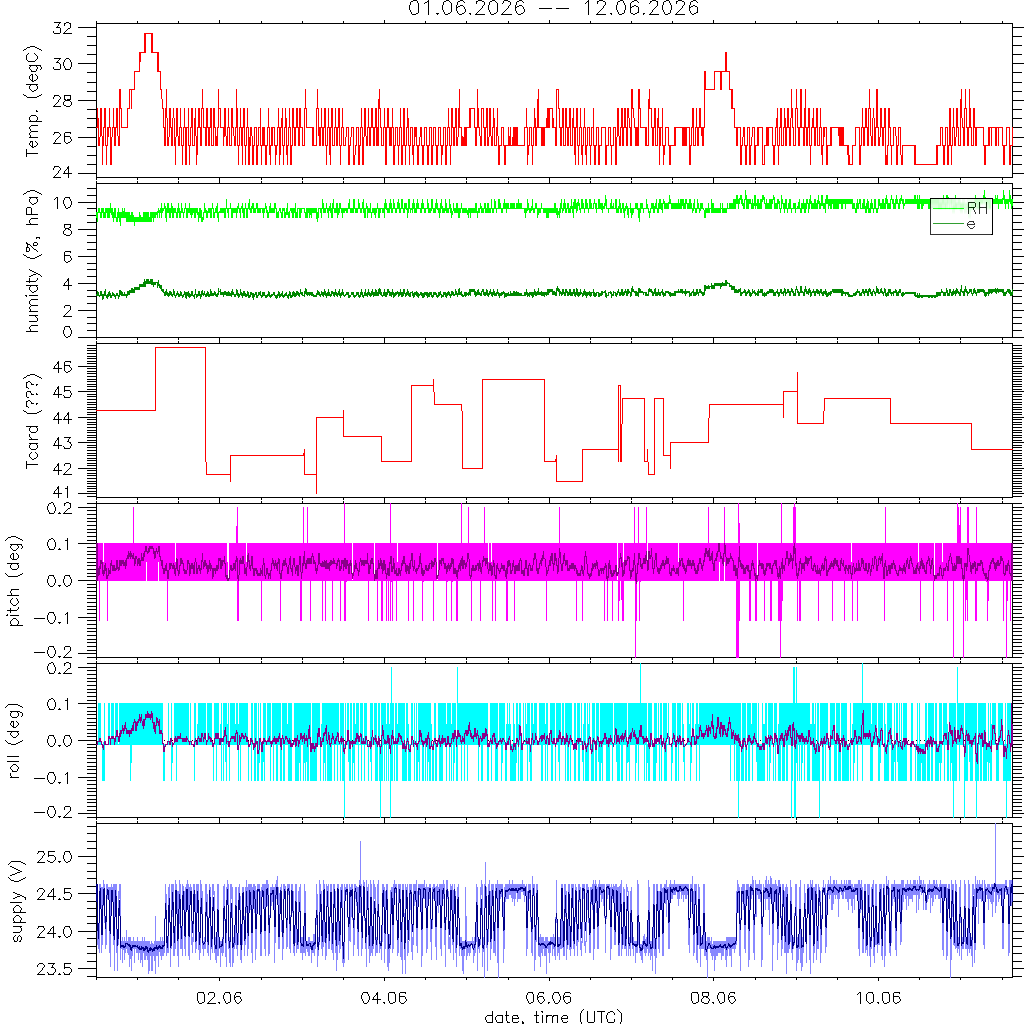
System log of its internal temperatur, humidity and power supply.
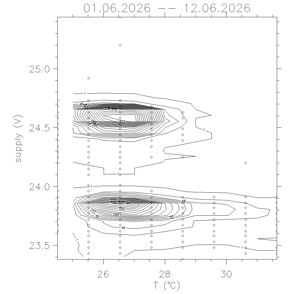
Volts versus power supply: both, when heating or cooling starts, supply goes down.
Cooling starts at 30degC, heating at 18.5degC.
Instruments goes into save mode (switch off) for temperatures above 41degC.
Arrows indicate gaps in time series and how temperatur and voltage changed.
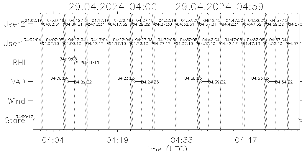
Schedule of the last hour.
Doppler velocity from 'VAD-36 - scan'
log beta from VAD-36 scan
Residuum after profile fit
Profiles from fit to VAD-36 - scan data
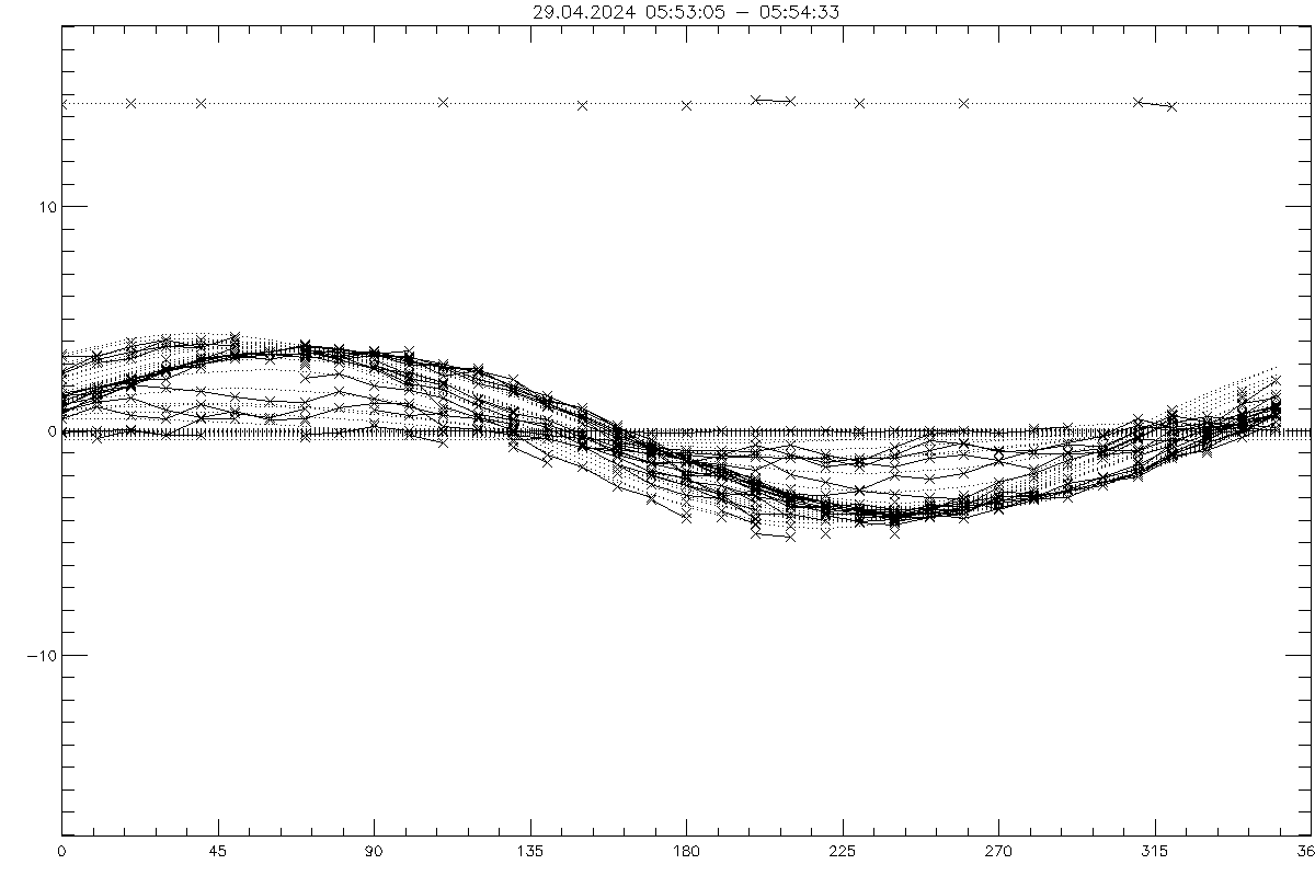
Doppler speeds in VAD-36 - scan versus azimuth and fits (dotted lines)
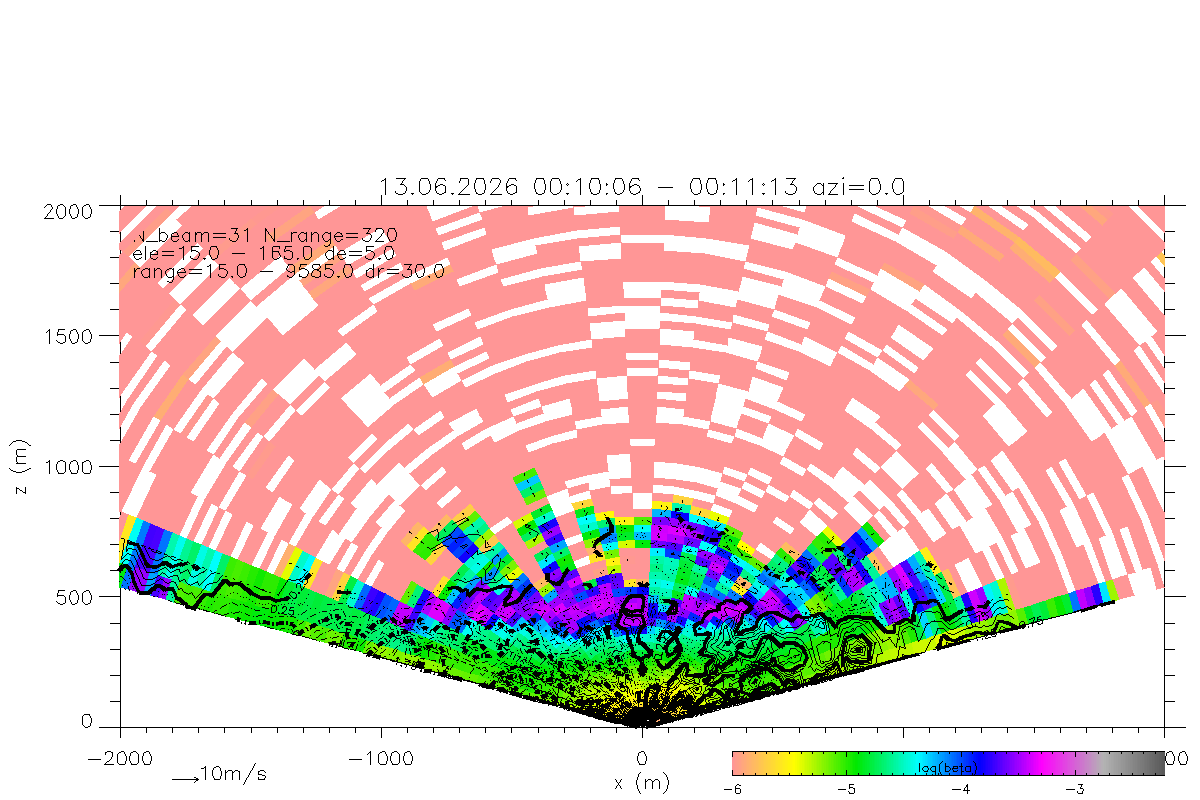
RHI scan with shading according to backscatter coeficient and measured doppler components along beam as vectors.

RHI scan with shading according to along beam doppler speeds.
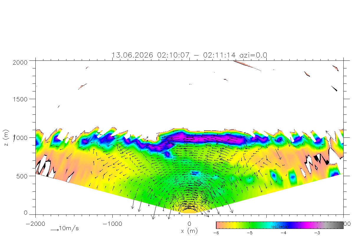
Plot of RHI scan with shading according to interpolated backscatter coeficient and wind vectors (u,w) in RHI plane based on a combination of two neighboring beams.
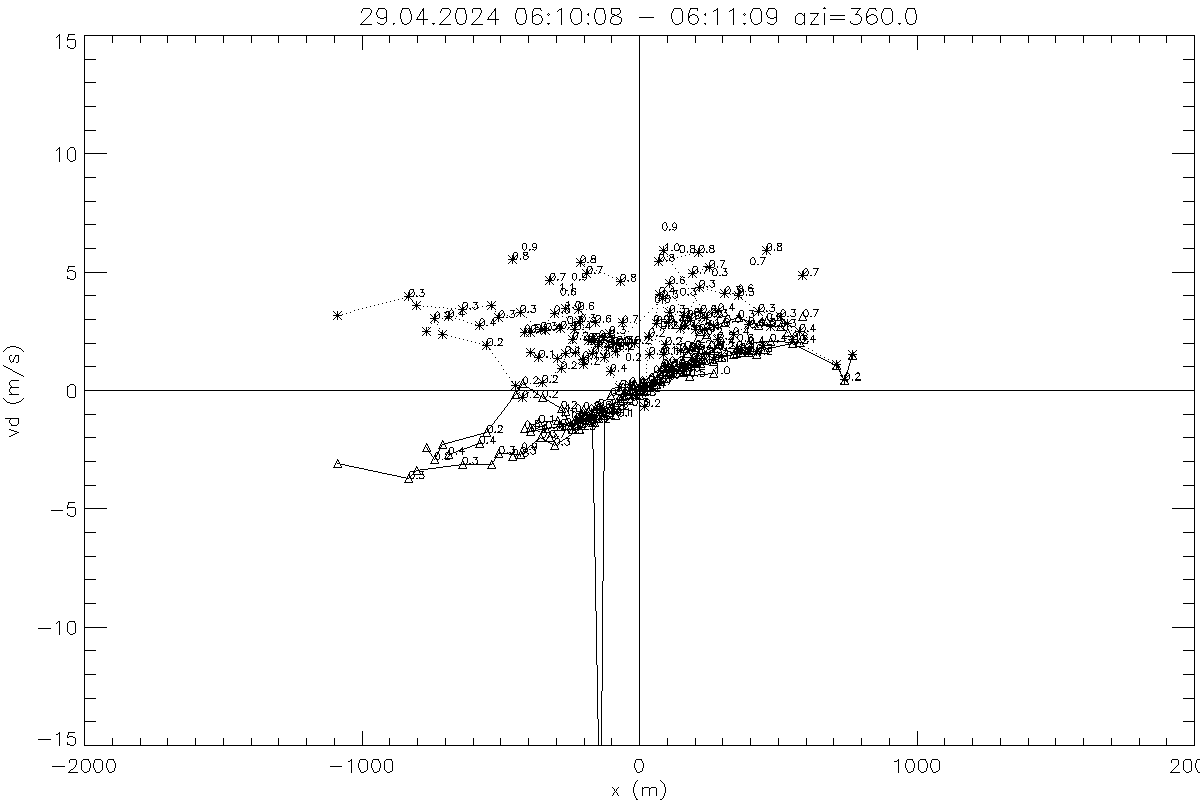
Doppler component vd along beam from RHI scan versus x-coordinate for different heights (solid lines triangles, height in km at data points),
and vd/cos(ele) = um + u' + w' tan(ele) (dotted line with asterisk) a measure for the average horizontal wind component um(z)
plus component due to deviation vector (u',w').