PAMTRA tutorial
PAMTRA overview
Model framework
PAMTRA as an acronym stands for Passive and Active Microwave TRAnsfer. It is a model framework written in FORTRAN90 and python for the simulation of passive and active RT (including Radar Doppler Spectra) in a plane-parallel, one-dimensional, and horizontally homogeneous atmosphere for the microwave frequency range up to 1 THz. With PAMTRA, the user is able to simulate up- and down-welling radiation at any height and observation angle in the atmosphere. The model framework includes several routines for reading and pre-processing of data from various input sources like cloud resolving models, profile measurements, or idealized profiles, e.g., designed for sensitivity studies. Due to its flexible design, a further extension for other input sources can be easily achieved.
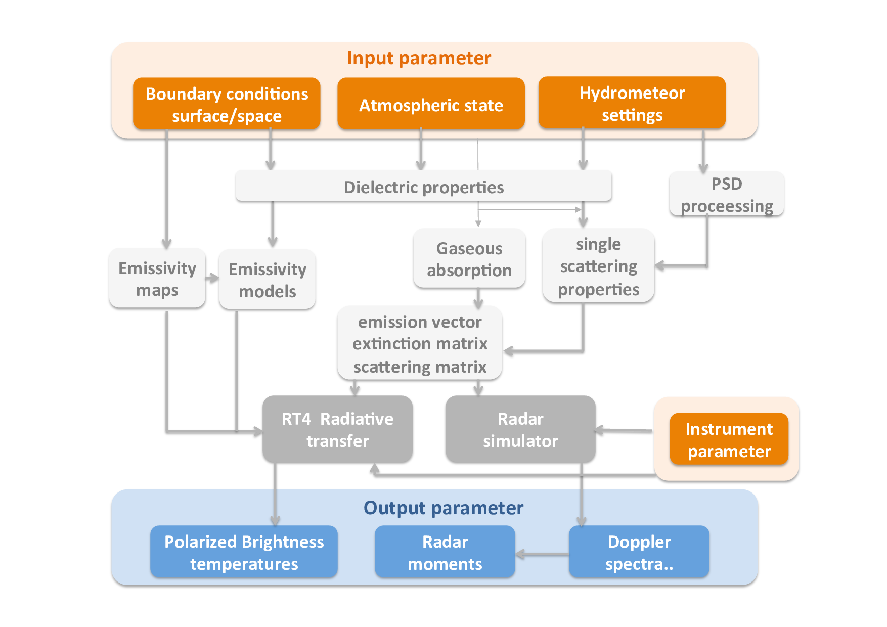
The flow diagram shows an overview of the various steps performed in the FORTRAN core of the present model setup. For the simulation, the model needs various inputs (shown in reddish colors):
- atmospheric state
- assumption on gaseous absorption
- assumption on hydrometeor single scattering properties
- boundary conditions, i.e., cosmic background surface emissivity
From these assumptions interaction parameters within various modules (white boxes) are generated. These parameters serve as input for the solving routines for the passive and active part (shown in gray). The simulations produce polarized radiances or TBs (brightness temperatures) for up- and down-welling geometries for arbitrary zenith angles and vertical and horizontal polarization for the passive part and radar Doppler spectra (and derived moments such as reflectivity, mean Doppler velocity, skewness, and kurtosis, as well as left and right slopes) for the active part.
pyPAMTRA adds a python framework around the FORTRAN core which allows to call PAMTRA directly from python without using the FORTRAN I/O routines. Consequently, pyPAMTRA is a more user-friendly way to access the PAMTRA model. It includes a collection of supporting routines, e.g. for importing model data or producing graphical output of the simulation results. With pyPAMTRA, a local parallel execution of PAMTRA on multi-core processor machines is possible. Furthermore, by using Python for I/O and flow control, interfacing PAMTRA to instrument or atmospheric models, as well as post-processing routines, is possible in a more comfortable way.
pyPamtra
The installation of PAMTRA is decribed within the PAMTRA documentation. Once the program has been compiled and the pyPamtra library is installed within your PYTHONPATH (e.g., $HOME/lib/python/) it can be used. Furthermore, it is helpfull to tell pamtra where it finds its auxiliary data by setting an environment variable PAMTRA_DATADIR
import sys
sys.path.append("/home/mech/lib/python/") # to find pyPamtra in case you did not install it yourself
import pyPamtra # main pamtra module
import os # import operating system module
# tell pamtra where itfinds its auxiliary data if not done before by the environment variable
os.environ['PAMTRA_DATADIR'] = '/net/sever/mech/pamtra/data/'
After importing pyPamtra, PAMTRA is available in your python environment. First step is to create a pyPamtra object.
pam = pyPamtra.pyPamtra() # basic empty pyPamtra object with default settings
pam.p
pam.nmlSet
Before we can proceed, pamtra needs definitions of hydrometeors. Up to now at least one is required to scale various arrays. This can be done by either directly define them:
pam.df.addHydrometeor(("ice", -99., -1, 917., 130., 3.0, 0.684, 2., 3, 1, "mono_cosmo_ice", -99., -99., -99., -99., -99., -99., "mie-sphere", "heymsfield10_particles",0.0))
or by importing the definitions from a file (examples are provided in descriptorfiles/ subdirectory).
pam.df.readFile(descriptorFilename)
No matter which way, in both cases at least one hydrometeor should now be defined.
pam.df.nhydro
Now it is time to provide pamtra some data. The mandatory atmospheric variables are
- hgt_lev (height levels) or hgt (height of layer means)
- temp_lev or temp
- press_lev or press
- relhum_lev or relhum
The following variables are optional and guessed if not provided: timestamp,lat,lon,lfrac,wind10u,wind10v,hgt_lev,hydro_q,hydro_n,hydro_reff,obs_height
These variables need to be stored in a python dictionary and can then be passed to the method to create a profile usable by pamtra.
pamData = dict()
pamData["temp"] = [275.,274.,273.]
pamData["relhum"] = [90.,90.,90.]
pamData["hgt"] = [500.,1500.,2500.]
pamData["press"] = [90000.,80000.,70000.]
pam.createProfile(**pamData) # create a pamtra profile.
# Produces a lot of warnings, just telling that many variables have been set to default
Another possibility to perform all these steps on standardized input is to use one of the importer methods provided by the pyPamtra package.
pam = pyPamtra.importer.readCosmoDe1MomDataset(...)
pam = pyPamtra.importer.readCosmoDe2MomDataset(...)
pam = pyPamtra.importer.readCosmoReAn2km(...)
pam = pyPamtra.importer.readCosmoReAn6km(...)
pam = pyPamtra.importer.readMesoNH(...)
pam = pyPamtra.importer.readWrfDataset(...)
These importer methods need various parameters,i.e like model output files and the appropriate descriptor file. Which parameters are necessary and accepted can be found out by:
pyPamtra.importer.readWrfDataset??
The profile used by pamtra is stored in the profile dictionary pam.p. What exactly is in there can be seen and inspected by
pam.p.keys() # gives a list of all entries of the dictionary
pam.p['temp'] # prints the temperature
The variables can still be changed before we later on perform the simulations.
Before we can run pamtra, it would be good to set some variables, so the model is doing what we want. What is set so far can be seen by examining the dictionary nmlSet:
pam.nmlSet
and the settings can be done by changing the members of that dictionary, i.e.:
pam.nmlSet['active'] = False # switch off active calculation
To perform a simulations, on of the methods pam.runPamtra() or pam.runParallelPamtra() needs to be applied. For the simple runPamtra method, only a frequency (or array of frequencies) needs to be provided.
pam.runPamtra(89.0)
If everything went fine and we got no errors or warnings, we should now have the results stored in the dictionary pam.r. Like for the profile dictionary pam.p, it can be inspected by pam.r.keys().
pam.r['tb'].shape # gives the shape of the calculated brightness temperature (tb) (nx,ny,noutlevels,nang,nfreq,npol)
pam.dimensions['tb'] # shows the dimensions
pam.r['tb'][0,0,0,0,0].mean(axis=-1)
# brightness temperature for satellite view in mixed polarization mode (mean of v and h)
As a final step the results can be either plotted, further examined, or stored to a netcdf file by a method provided by pamtra:
pam.writeResultsToNetCDF('example.nc')
from __future__ import division # defines natural divisions like 1./2. = 1/2 = 0.5 and not 1/2 = 0
import sys
sys.path.append("/home/mech/lib/python/") #to find pyPamtra
import pyPamtra  # import pyPamtra
import matplotlib.pyplot as plt  # import ploting modules
import numpy as np # import numpy for arrays, numerical array operations, ....
import pandas as pn # import pandas data analysis library
import os # import operating system module
os.environ['PAMTRA_DATADIR'] = '/met/sever/mech/pamtra/data/'
%matplotlib inline
Create a pyPamtra object
pam = pyPamtra.pyPamtra()
Define the hydrometeor classes. Replace "mie-sphere" by "disabled" to turn off hydrometeor. Everything in SI units!
descriptorFile = np.array([
      #['hydro_name' 'as_ratio' 'liq_ice' 'rho_ms' 'a_ms' 'b_ms' 'alpha_as' 'beta_as' 'moment_in' 'nbin' 'dist_name' 'p_1' 'p_2' 'p_3' 'p_4' 'd_1' 'd_2' 'scat_name' 'vel_size_mod' 'canting']
       ('cwc_q', -99.0, 1, -99.0, -99.0, -99.0, -99.0, -99.0, 3, 1, 'mono', -99.0, -99.0, -99.0, -99.0, 2e-05, -99.0, 'mie-sphere', 'khvorostyanov01_drops', -99.0),
       ('iwc_q', -99.0, -1, -99.0, 130.0, 3.0, 0.684, 2.0, 3, 1, 'mono_cosmo_ice', -99.0, -99.0, -99.0, -99.0, -99.0, -99.0, 'mie-sphere', 'heymsfield10_particles', -99.0),
       ('rwc_q', -99.0, 1, -99.0, -99.0, -99.0, -99.0, -99.0, 3, 50, 'exp', -99.0, -99.0, 8000000.0, -99.0, 0.00012, 0.006, 'mie-sphere', 'khvorostyanov01_drops', -99.0),
       ('swc_q', -99.0, -1, -99.0, 0.038, 2.0, 0.3971, 1.88, 3, 50, 'exp_cosmo_snow', -99.0, -99.0, -99.0, -99.0, 5.1e-11, 0.02, 'mie-sphere', 'heymsfield10_particles', -99.0),
       ('gwc_q', -99.0, -1, -99.0, 169.6, 3.1, -99.0, -99.0, 3, 50, 'exp', -99.0, -99.0, 4000000.0, -99.0, 1e-10, 0.01, 'mie-sphere', 'khvorostyanov01_spheres', -99.0)],
      dtype=[('hydro_name', 'S15'), ('as_ratio', '<f8'), ('liq_ice', '<i8'), ('rho_ms', '<f8'), ('a_ms', '<f8'), ('b_ms', '<f8'), ('alpha_as', '<f8'), ('beta_as', '<f8'), ('moment_in', '<i8'), ('nbin', '<i8'), ('dist_name', 'S15'), ('p_1', '<f8'), ('p_2', '<f8'), ('p_3', '<f8'), ('p_4', '<f8'), ('d_1', '<f8'), ('d_2', '<f8'), ('scat_name', 'S15'), ('vel_size_mod', 'S30'), ('canting', '<f8')]
      )
Table as panda DataFrame
pn.DataFrame(descriptorFile)
for hyd in descriptorFile: pam.df.addHydrometeor(hyd)
#pam.df.readFile('/home/mech/workspace/pamtra/descriptorfiles/descriptor_file.txt')
pam.df.nhydro
pam.readPamtraProfile('/home/mech/workspace/pamtra/profile/example_input.lay')
fig = plt.figure(figsize=[12,4])
fig.add_axes([0.1,0.1,0.25,0.8])
plt.plot(pam.p['press'][0,0,:]/100.,pam.p['hgt'][0,0,:])
plt.ylabel('height [m]')
plt.xlabel('pressure [hPa]')
fig.add_axes([0.425,0.1,0.25,0.8])
plt.plot(pam.p['temp'][0,0,:],pam.p['hgt'][0,0,:])
plt.xlabel('temperature [K]')
fig.add_axes([0.75,0.1,0.25,0.8])
plt.plot(pam.p['relhum'][0,0,:],pam.p['hgt'][0,0,:])
plt.xlabel('rel. humidity [%]')
plt.show()

freqs = np.arange(10.,200.,1.)
freqs
pam.runParallelPamtra(freqs, pp_deltaX=1, pp_deltaY=1, pp_deltaF=10, pp_local_workers="auto")
pam.r["tb"].shape # ngridx,ngridy,noutlevel,nangles,nfreqs,npol
plt.figure()
plt.plot(freqs,pam.r["tb"][0,0,0,0,:,0],label='upwelling T$_\mathrm{B}$')
plt.plot(freqs,pam.r["tb"][0,0,1,31,:,0],label='downwelling T$_\mathrm{B}$')
plt.xlabel('frequency [GHz]')
plt.ylabel('brightness temperature [K]')
plt.legend(loc=4)
plt.show()

pam.writeResultsToNetCDF('example_spectrum.nc')
Simulate a radiometer measurement from a radiosonde observation
First load a bunch of libraries
# -*- coding: utf-8 -*-
from __future__ import division
import numpy as np
import matplotlib.pyplot as plt
import pyPamtra
import pandas as pn
import netCDF4
import socket

#%matplotlib inline
read the radiosonde
rsData = netCDF4.Dataset("/home/mech/workspace/pamtra/doc/tutorials/data/rsdata.nc")
rsData.variables.keys()
Create pyPamtra object
pam = pyPamtra.pyPamtra()
As of now, Pamtra needs at least one Hydrometeor type, we discuss the details later
pam.df.addHydrometeor(("ice", -99., -1, 917., 130., 3.0, 0.684, 2., 3, 1, "mono_cosmo_ice", -99., -99., -99., -99., -99., -99., "mie-sphere", "heymsfield10_particles",0.0))
#pam.df.data
#pn.DataFrame(pam.df.data)
Collect the data required by Pamtra
pamData = dict()
pamData["temp"] = rsData.variables["air_temperture"][:] + 273.15
pamData["press"] = rsData.variables["air_pressure"][:]
pamData["relhum"] = rsData.variables["relative_humidity"][:] * 100
pamData["hgt"] = rsData.variables["height"][:]
Optional data
pamData["lat"] =rsData.variables["latitude"][:]
pamData["lon"] =rsData.variables["longitude"][:]
pamData["lfrac"] = np.array([1])
pass the data to the pamtra object. Note how additonal data is added
pam.createProfile(**pamData)
equivalent to: pam.createProfile(temp=pamData["temp"],relhum?pamData["relhum"],....)
Settings
pam.nmlSet
pam.nmlSet["active"] = False
That's it!. Run Pamtra
pam.runPamtra([22.24,51.26])
Explore the results
pam.r["tb"]
print pam.dimensions["tb"]
print pam.p["obs_height"]
print pam.r["angles_deg"]
gridx = 0
gridy = 0
outlevel = 1
angle= np.where(pam.r["angles_deg"]==0)[0] # gives the index where angles_deg == 0
groundbased zenith view
pam.r["tb"][gridx,gridy,outlevel,angle].mean(axis=-1)
satellite nadir view
outlevel = 0
angle= np.where(pam.r["angles_deg"]==180)[0]
pam.r["tb"][gridx,gridy,outlevel,angle].mean(axis=-1)
run pamtra parallel
f_hatpro_Kband = [22.24, 23.04, 23.84, 25.44, 26.24, 27.84, 31.40]
f_hatpro_Vband = [51.26, 52.28, 53.86, 54.94, 56.66, 57.30, 58.00]
pam.runParallelPamtra(f_hatpro_Kband+f_hatpro_Vband,pp_local_workers='auto', pp_deltaF=1, pp_deltaX=0, pp_deltaY=0)
gridx = 0
gridy = 0
outlevel = 1
angle= np.where(pam.r["angles_deg"]==0)[0]
pam.r["tb"][gridx,gridy,outlevel,angle].mean(axis=-1)
plt.plot(pam.r["tb"][gridx,gridy,outlevel,angle].mean(axis=-1).flatten())
plt.xticks(range(len(pam.set["freqs"])),pam.set["freqs"],rotation=90)
plt.show()

pam.writeResultsToNetCDF("pamtra_rs.nc")
Simulate a CloudSat measurement from a Como field
from __future__ import division
import numpy as np
import matplotlib.pyplot as plt
import matplotlib
import pandas as pn
import pyPamtra

#%matplotlib inline
define the hydrometeor classes. Replace "mie-sphere" by "disabled" to turn off a specfic hydrometeor. Everything in SI units!
descriptorFile = np.array([
      #['hydro_name' 'as_ratio' 'liq_ice' 'rho_ms' 'a_ms' 'b_ms' 'alpha_as' 'beta_as' 'moment_in' 'nbin' 'dist_name' 'p_1' 'p_2' 'p_3' 'p_4' 'd_1' 'd_2' 'scat_name' 'vel_size_mod' 'canting']
       ('cwc_q', -99.0, 1, -99.0, -99.0, -99.0, -99.0, -99.0, 3, 1, 'mono', -99.0, -99.0, -99.0, -99.0, 2e-05, -99.0, 'mie-sphere', 'khvorostyanov01_drops', -99.0),
       ('iwc_q', -99.0, -1, -99.0, 130.0, 3.0, 0.684, 2.0, 3, 1, 'mono_cosmo_ice', -99.0, -99.0, -99.0, -99.0, -99.0, -99.0, 'mie-sphere', 'heymsfield10_particles', -99.0),
       ('rwc_q', -99.0, 1, -99.0, -99.0, -99.0, -99.0, -99.0, 3, 50, 'exp', -99.0, -99.0, 8000000.0, -99.0, 0.00012, 0.006, 'mie-sphere', 'khvorostyanov01_drops', -99.0),
       ('swc_q', -99.0, -1, -99.0, 0.038, 2.0, 0.3971, 1.88, 3, 50, 'exp_cosmo_snow', -99.0, -99.0, -99.0, -99.0, 5.1e-11, 0.02, 'mie-sphere', 'heymsfield10_particles', -99.0),
       ('gwc_q', -99.0, -1, -99.0, 169.6, 3.1, -99.0, -99.0, 3, 50, 'exp', -99.0, -99.0, 4000000.0, -99.0, 1e-10, 0.01, 'mie-sphere', 'khvorostyanov01_spheres', -99.0)],
      dtype=[('hydro_name', 'S15'), ('as_ratio', '<f8'), ('liq_ice', '<i8'), ('rho_ms', '<f8'), ('a_ms', '<f8'), ('b_ms', '<f8'), ('alpha_as', '<f8'), ('beta_as', '<f8'), ('moment_in', '<i8'), ('nbin', '<i8'), ('dist_name', 'S15'), ('p_1', '<f8'), ('p_2', '<f8'), ('p_3', '<f8'), ('p_4', '<f8'), ('d_1', '<f8'), ('d_2', '<f8'), ('scat_name', 'S15'), ('vel_size_mod', 'S30'), ('canting', '<f8')]
      )
Table looks better when converting it to a DataFrame
pn.DataFrame(descriptorFile)
Use the Cosmo import routine to read Comso netCDF
constantFields = "/home/mech/workspace/pamtra/doc/tutorials/data/cosmo_constant_fields.nc"
fname='/home/mech/workspace/pamtra/doc/tutorials/data/LMK_gop9_test_fields_SynSatMic_201307241200-0900.nc.gz'
pam = pyPamtra.importer.readCosmoDe1MomDataset(fname,"gop_fields_SynSatMic",descriptorFile,colIndex=0,verbosity=1,constantFields=constantFields)
Settings
#turn off passive calculations
pam.nmlSet["passive"] = False
#used frequencies
frequencies = [94]

#show some messages
pam.set["verbose"] = 0
pam.set["pyVerbose"] = 1
Cut out the CloudSat track and remove from the pamtra object
filterPam = np.zeros(pam._shape2D,dtype=bool)
filterPam[3:400,240] = True
print pam._shape3D
pam.filterProfiles(filterPam)
print pam._shape3D
Run Pamtra
W-band is attenuated
pam.nmlSet['radar_attenuation'] = 'top-down'
pam.runParallelPamtra(frequencies, pp_deltaX=1, pp_deltaY=1, pp_deltaF=0, pp_local_workers="auto")
store results
outName = "cosmo_field_20130724_94.nc"
pam.writeResultsToNetCDF(outName, ncForm='NETCDF3_CLASSIC')
pam.r["Ze"]
pam.dimensions["Ze"]
frequency = 0
radar_npol = 0
gridy = 0
radar_npeak = 0
Ze = pam.r["Ze"][:,gridy,:,frequency,radar_npol,radar_npeak]
H = pam.p["hgt"][:,gridy]
lon = pam.p["lon"][:,gridy]
matplotlib.rcParams['figure.figsize'] = (10.0, 8.0)
plt.pcolormesh(lon,H.T,Ze.T,vmin=-50,vmax=30)
plt.ylim(0,np.max(H))
plt.xlim(np.min(lon),np.max(lon))
plt.xlabel("longitude [deg]")
plt.ylabel("height [m]")
plt.colorbar(label="Ze [dBz]")
plt.show()

PAMTRA on Oberschleissheim radiosonde in comparison to HALO EMV flight observations
Read in the radiosonde data. The file has been modified to make is easier.
import numpy as np
rsData = np.genfromtxt('data/oberschleissheim_2016071912.txt',comments='#',skip_header=3,names=True)
import pyPamtra and create an pyPamtra object
import pyPamtra
pam = pyPamtra.pyPamtra()
It is mandatory to add a hydrometeor, eventhough it might be a clear sky profile.
pam.df.addHydrometeor(("ice", -99., -1, 917., 130., 3.0, 0.684, 2., 3, 1, "mono_cosmo_ice", -99., -99., -99., -99., -99., -99., "mie-sphere", "heymsfield10_particles",0.0))
Put the radiosonde data in a dictionary.
pamData = dict()
pamData["temp"] = rsData["TEMP"][:] + 273.15
pamData["press"] = rsData["PRES"][:] *100.
pamData["relhum"] = rsData["RELH"][:]
pamData["hgt"] = rsData["HGHT"][:]
pamData["lat"] = np.array([48.25])
pamData["lon"] = np.array([11.55])
pamData["lfrac"] = np.array([1])
pam.createProfile(**pamData)
pam.p.keys()
pam.runPamtra(22.24)
pam.r.keys()
pam.r['tb']